[논문리뷰] C2AE: Class Conditioned Auto-Encoder for Open-set Recognition

Paper Overview

CVPR'19

https://arxiv.org/abs/1904.01198

C2AE: Class Conditioned Auto-Encoder for Open-set Recognition

 

Abstract

 

신경망 모델에 unknown example이 입력되면 일반적으로 어느 한 class로 분류하게 된다.

이를 해결하기 위해 Open-set recognition은 입력 data 중 unknown을 구별하고

known만을 분류하여 모델 성능을 유지하는 task다.

이 task는 training동안 world의 불완전한 지식 때문에 unknown sample을 찾아내는 것이 어렵다.

(특히 학습에는 known class만 사용가능하기 때문.)

저자들은 novel training, testing methodology를 통해 conditioned auto-encoder를 사용하는

open-set recognition algorithm을 제안한다.

training 절차는 2가지 sub-task로 나뉜다.

1. closed-set classification

2. open-set identification

Encoder는 closed-set classification training을 따라 first task를 학습하고

반면에 decoder는 class identity를 조건으로 reconstructng을 함으로써 second task를 학습한다.

 

Keywords

Open-set Recognition, VAE

---

Proposed Method

저자들의 프레임워크는 다음과 같다.

 

3.1 Closed-set Training (Stage 1)

 

한 배치 $\left\{X_{1}, X_{2}, ..., X_{N}\right\} \in K$ 가 주어지면

대응되는 label은 $\left\{X_{1}, X_{2}, ..., X_{N}\right\}$이다.

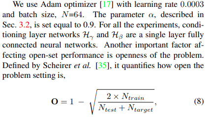
$N$은 batch size이고 $\forall y_{i} \in \left\{ 1,2,...,k\right\}$이다.

encoder $F$와 classifier $C$는 파라미터 $\theta_{f}$와 $\theta_{c}$로 구성되고

cross entropy loss에 의해 학습된다.

$\mathbb{I}_{y_{i}}$는 label $y_i$에 대한 indicator function이다.

(one-hot)

 

3.2 Open-set Training (Stage 2)

 

Conditional Decoder Training

 

$F$는 latent vector를 추출하는데 사용될 수 있다. $\left\{z_{1}, z_{2}, ..., z_{N}\right\}$

이 latent vector batch는 FiLM에 의해 조건화 된다.

FiLM은 Feature-wise Linear Moduation을 적용함으로써

input feature map에 conditioning information 영향을 준다.

input feature $z$와 conditioning information이 포함된 vector $l_{j}$가 주어지면,

다음과 같이 표현할 수 있다.

 

$H_\gamma$, $H_\beta$는 파라미터 $\theta_\gamma$, $\theta_\beta$로 구성된 신경망이다.

$z_{l_{j}}$, $\gamma_{j}$, $\beta_{j}$는 같은 shape다.

$\odot$는 Hadamard product(=elements-wise product)를 나타낸다.

 

decoder $mathcal{G}$는 label condition vector가 input class identity와 매칭되면

완벽하게 original input을 reconstruct한다고 기대한다.

그러나 $mathcal{G}$는 추가적으로 match가 안되는 condition을

잘못 reconstruct하도록 학습된다.

이때 제대로된 condition은 $l_{m}$이라 하고 잘못된 condition을 $l_{nm}$이라 한다.

 

한 input $X_{i}$에 대해 match $m$, non-match $nm$의

feed forward path는 다음과 같이 요약할 수 있다.

따라서 loss function을 다음과 같이 작성할 수 있다.

이 방법은 $l_{y_{i}^{nm}}$이 주어질 때 잘못된 reconstruction을 하도록 할 수 있다.

그래서 unknown class test sample이 입력될 때,

이상적으로 어떤 condition이든 $l_{nm}$이므로 잘못된 reconstruction이 될 것이다.

이때 $\alpha$는 0~1 값이다.

 

EVT Modeling

 

Extreme Value Theory

 

저자들은 extreme value theory의 Picklands-Balkema-deHaan formulation를 따른다.

위키백과에 나온 내용은 다음과 같다.

The Pickands–Balkema–De Haan theorem gives the asymptotic tail distribution of a random variable, when its true distribution is unknown

이것은 high threshold를 초과하는 random variable에 조건으로 하는 probability를 모델링한다.

random variable $W$가 cumulative distribution function(CDF) $F_{W}(w)$와 주어지면,

threshold $u$를 초과하는 어떤 $w$에 대한 conditional CDF는 다음과 같이 정의할 수 있다.

 

이제, Independent and Identically Distribution (IID) sample $\left\{W_{i}, ...,W_{n}\right\}$가 주어지면

extreme value theorem은 $F_U$가 Generalized Pareto Distribution (GPD)로 근사될 수 있다고 한다.

$-\infty < \zeta < +\infty$, $0 < \mu < +\infty$, $w>0$, $\zeta w > -\mu$다.

$G(\cdot)$은 GPD의 CDF다.

 $\zeta = 0$에 대해 parameter $\mu$에 대한 지수 분포로 축소된다.

$\mu \neq 0$에 대해 Pareto distribution이 된다.

 

Parameter Estimation

 

어떤 분포의 tail이든 GPD로 모델링 할 때

주된 어려움은 tail parameter $u$를 찾는 것이다.

그러나 $u$의 값을 추정하는 것은 mean excess function (MEF)를 사용하여 가능하다.

($E\left[W-u|W>u\right]$)

GPD, MEF는 $u$의 선형 관계에 있다.

이것을 추정하는 방법은 다음 논문을 참고하면 된다.

Extreme value analysis for mobile active user authentication
Modeling biometric systems using the general pareto distribution (gpd)

또 나머지 파라미터($\mu$, $\zeta$)는 maximum likelihood estimation을 통해 쉽게 구할 수 있다.

 

Threshold Calculation

 

$r_{i}^{m}$은 match reconstruction error이고

$r_{i}^{nm}$은 non match reconstruction error이다.

이는 다음과 같이 계산할 수 있다.

 

히스토그램 $S_M$과 $S_{nm}$은 다음과 같다.

 

이때 $S_M$과 $S_{nm}$이 잘 근사된 것을 확인할 수 있다.

 

optimal operating threshold ($\tau^{*}$)는 $S_{m}\cap S_{nm}$에 놓여있다고 가정할 수 있다.

(이 영역은 위 Fig.3에서 보이는 겹치는 영역이다.)

$S_m$의 tail(left tail)과 $S_{nm}$의 tail(right tail)을 GPD의 $G_m$, $G_{nm}$으로 모데링하는 것이 가능하다.

GPD는 maxima modeling에 대해서만 정의하므로, $S_{nm}$의 left tail을 $G_{nm}$으로 fitting하기 전에

저자들은 inverse transform을 $S'_{nm} = -S_{nm}$으로 변환한다.

unknown sample을 관측하는 것의 prior probability는 $p_u$라 가정하면

error의 probability는 $\tau$로 공식화 할 수 있다.

 

3.3 Open-set Testing by k-inference (Stage3)

 

이 testing strategy는 $k$번 반복한다.

---

Experiments

1. Implementation Details

 

 

 

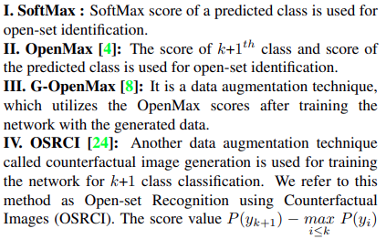
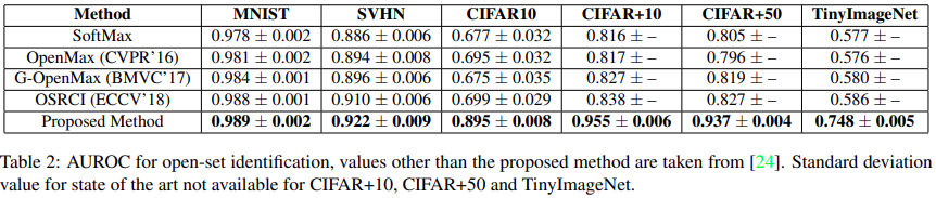
2. Experiment $\mathbb{I}$ :  Open-set Identification

Dataset

 

MNIST, SVHN, CIFAR10

openset 13.39%

 

CIFAR+10, CIFAR+50

open set 33.33%

 

TinyImageNet

open set 57.35%

 

Comparision with state-of-the-art

 

---

Conclusion

We presented an open-set recognition algorithm based on class conditioned auto-encoders. We introduced training and testing strategy for these networks. It was also shown that dividing the open-set recognition into sub tasks helps learn a better score for open-set identification. During training, enforcing conditional reconstruction constraints are enforced, which helps learning approximate known and unknown score distributions of reconstruction errors. Later, this was used to calculate an operating threshold for the model. Since inference for a single sample needs k feed-forwards, it suffers from increased test time. However, the proposed approach performs well across multiple image classification datasets and providing significant improvements over many state of the art open-set algorithms. In our future research, generative models such as GAN/VAE/FLOW can be explored to modify this method. We will revise the manuscript with such details in the conclusion.